
Occupancy Inference from Aggregate Smart-Meter Data Across Sampling Resolutions: A Controlled Synthetic
Abstract
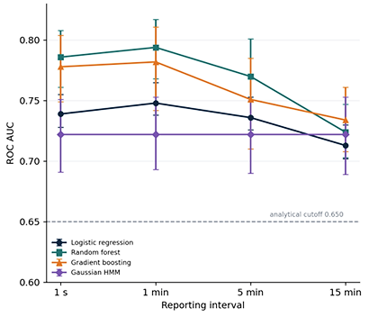
Fine-grained smart-meter records support legitimate energy services while also enabling behavioral inference. This study isolates one controllable disclosure parameter—the reporting interval—and examines how it changes retrospective occupancy inference in a controlled synthetic benchmark. Sixty households are simulated for 14 days at one-second native resolution, then mean-aggregated to 1-second, 1-minute, 5-minute, and 15-minute releases. Non-overlapping 30-minute windows are represented by statistical and temporal features and evaluated with logistic regression, random forest, gradient boosting, and a two-state Gaussian Hidden Markov Model (HMM). The primary protocol trains on 42 households and evaluates 18 previously unseen households (12,096 windows); uncertainty is summarized by a 500-draw household-cluster bootstrap. Random forest attains its highest pooled Receiver Operating Characteristic – Area Under the Curve (ROC AUC) at 1 minute (0.794; 95% bootstrap interval 0.768–0.817) and declines to 0.724 (0.703–0.747) at 15 minutes. Gradient boosting reaches 0.734 (0.708–0.761) at 15 minutes. Statistical-only feature sets consistently outperform temporal-only sets, showing that coarse releases can retain occupancy-linked level information after short transitions are suppressed. The HMM remains at AUC 0.722 at every resolution because it receives only the 30-minute mean, which is invariant under the nested averaging scheme. The analysis also exposes three interpretive boundaries: The midpoint label is estimated using the complete window and is therefore retrospective; a secondary time split changes several design factors and cannot identify the causal value of household-specific history; and the AUC 0.650 line is an analytical benchmark rather than a legal or operational privacy threshold. The findings support data minimization as a useful but incomplete control: 15-minute averaging reduces some model performance without eliminating inferential exposure in this generator. External validation on occupancy-labeled homes, prospective inference, and release of code, generated traces, predictions, and bootstrap draws are required before deployment claims.
Keywords:Smart meterOccupancy inferenceData granularityPrivacy exposureSynthetic simulationHousehold-cluster
bootstrap.
1. Introduction
Advanced metering infrastructure changes an electricity meter from a periodic billing device into a longitudinal sensor of household activity. Aggregate power traces contain switching events, persistent base loads, appliance cycles, and time-of-day structure. These signals made non-intrusive load monitoring possible [1], but the same observability creates a privacy problem: A record collected for billing, forecasting, or demand response may also support inferences about appliance use, routines, and presence at home [2–4]. The privacy risk is therefore not confined to direct identifiers. It also arises from what a capable analyst can infer after the meter record has been released, linked, or retained.
Occupancy is a particularly consequential inference target. Presence information can be useful for demand-side management and building control, yet repeated estimates of absence can reveal daily schedules. Prior studies have shown that consumption statistics can support occupancy classification in small residential deployments [5–8], communication-oriented attack settings [9], and large populations [10]. These studies differ in sensing frequency, ground-truth construction, window definition, model family, and train–test separation. Consequently, a single reported accuracy does not answer the policy question of how much exposure remains after data are temporally aggregated.
Sampling resolution is attractive as a data-minimization control because it can be implemented before release and is easy to explain. Coarser intervals suppress short-lived transitions and reduce record volume. They do not necessarily remove persistent level differences, duty cycles, or routine structure. Eibl and Engel [11] demonstrated that granularity affects appliance-edge detection, while later work showed that sampling frequency can materially alter summary features of household load profiles [12]. The practical question is therefore not whether coarsening discards information—it must—but which information remains available to a specified adversary and whether that residual signal still supports the sensitive inference of interest. The present study treats reporting interval as the controlled factor in a synthetic benchmark. The same native one-second traces are averaged to four release intervals, the same 30-minute analysis window is retained, and a common set of classifiers is evaluated on households excluded from model training. This design is valuable because it separates the mechanical effect of temporal aggregation from changes in the underlying household sample. It is also deliberately limited: The generator constructs the relationship between occupancy and consumption, so absolute Area Under the Curve (AUC) values cannot be transported to real households without external validation. The experiment should be read as a controlled stress test of an inference channel, not as a universal privacy certification.
We make four contributions: 1) we position resolution-aware occupancy inference within the broader smart-meter privacy literature and separate attack measurement from privacy protection. 2) we state an explicit archived-trace threat model and expose the temporal information available at the midpoint label. 3) we compare four classifiers and two feature families under a household-disjoint protocol with cluster-aware uncertainty. 4) we explain two important invariances and confounds: The 30-minute mean presented to the Hidden Markov Model (HMM) is mathematically unchanged by nested averaging, whereas the secondary time split changes several design dimensions at once. These clarifications make the results more useful for data-release decisions while preserving the boundary between observed evidence and proposed future validation. The timeline is illustrative rather than a systematic-review flow diagram; it identifies the line of work to which the controlled resolution experiment contributes.
This figure is shown in the PDF version of the article.
2. Background and Related Work
2.1 From Appliance Signatures to Behavioral Inference
Hart’s [1] formulation of non-intrusive appliance load monitoring established that aggregate demand can be decomposed by exploiting characteristic transitions and operating states. Subsequent privacy work reversed the perspective: Features useful for energy feedback may also reveal personal information. Molina-Markham et al. [2] described the meter trace as a behavioral record whose fine detail can expose activities, while Lisovich et al. [3] analyzed how demand-response data can disclose private attributes and routines. McKenna et al. [4] framed the resulting governance problem as a balance between legitimate system applications and data minimization. This dual-use structure remains central: The same statistical regularities can support operational efficiency under authorized use and intrusive inference under secondary or unauthorized use.
Inference need not recover individual appliances to create exposure. Smart-meter records have been used to estimate household characteristics from consumption shape [5] and to fingerprint households across weekly excerpts [13]. Such results show why pseudonymization alone is not a complete defense: Repeated load patterns may act as quasi-identifiers. Occupancy is similarly inferential. Chen et al. [6] linked short-window load statistics to presence in two homes. Kleiminger et al. [7], [8] evaluated occupancy classification from electricity traces and later developed household occupancy monitoring using meter data. Tang et al. [9] demonstrated non-intrusive occupancy detection from load curves, and Razavi et al. [10] extended the question to more than 5,000 households with machine-learning feature engineering. Collectively, this literature establishes feasibility but also underscores heterogeneity across homes and protocols.
2.2 Resolution, Feature Survival, and Privacy–Utility Trade-Offs
Temporal aggregation is often treated as a monotone privacy control: If the reporting interval increases, sensitive information is expected to decrease. The premise is directionally sensible but incomplete. Averaging acts as a low-pass operation. A short switching edge can disappear, yet a sustained increase in demand remains visible in the window mean, minimum, or occupancy-conditioned base level. Eibl and Engel [11] quantified the relationship between granularity and appliance-edge detection. Hernandez et al. [12] showed that sampling frequency changes load-profile features and that feature sensitivity varies across metrics. These findings motivate feature-family analysis rather than a single full-model comparison.
Privacy reviews organize available defenses into data manipulation, cryptographic aggregation, differential privacy, and physical demand shaping using storage or controllable loads [14–18]. Down-sampling belongs to data minimization: It changes what leaves the meter but does not provide a formal privacy guarantee. Differential privacy can provide a defined guarantee for an explicit query mechanism, yet its utility depends on the released statistic, population size, and privacy budget; real smart-meter deployments can be challenging [19]. Battery-based masking and load scheduling operate at a different layer by changing the observable demand profile. The present study evaluates exposure after aggregation only. It does not test a protection mechanism under adversarial retraining, and it does not estimate a formal privacy parameter.
2.3 Synthetic Demand Models and External Validity
Synthetic traces are useful when occupancy ground truth is unavailable or privacy-sensitive. Established residential demand models use time-use surveys, Markov occupancy processes, and appliance-level bottom-up simulation to reproduce high-resolution variation [20–22]. Their scientific value depends on transparent generator assumptions and validation against measured populations. A synthetic benchmark can identify whether a method is internally coherent and can support controlled counterfactual changes. It cannot, by itself, estimate how often an effect occurs in heterogeneous real homes, where photovoltaic generation, electric vehicles, heating and cooling, household composition, and behavior may change both the signal and the class balance.
The distinction is especially important for occupancy research. Reviews of building occupancy detection show that performance depends on sensor modality, building type, label source, evaluation horizon, and transfer setting [23]. A model that performs well when the same household contributes training history answers a different question from a model transferred to an unseen household. Likewise, a retrospective classifier using a complete window answers a different question from an online detector at the window midpoint. We therefore use design descriptors—data source, temporal direction, household overlap, and inference target— as part of the result, not as secondary implementation details.
Table 1. Representative literature and the specific gap addressed by the present experiment.
This table is shown in the PDF version of the article.
3. Threat Model, Scope, and Research Questions
We consider an analyst who obtains a longitudinal aggregate active-power record for a household at a declared reporting interval. The analyst does not observe appliance submetering or the true occupancy state, but has labeled synthetic households from the same generator and can train a classifier. The primary adversary must transfer to households that were absent from training. The task is to rank whether the home was occupied at the midpoint of each 30-minute interval. This is an archived-trace scenario: the complete 30-minute window is available, and the HMM uses smoothed posteriors over the sequence. It is not a real-time alarm evaluated at minute 15.
Let xh(t) denote the native aggregate power of household h and oh(t) its binary simulated occupancy. For release interval Δ, the disclosed series is the non-overlapping average AΔ{xh(t)}. A feature map φ is applied to the values inside window w, and the label is the state at the midpoint of that window.
zh (Δ ,v) = φ(AΔ{xh(t): t ∈ [τv, τv + 30 min)}), yh,v = oh(τv + 15 min).
A model produces a score s(z) and is evaluated by the pooled area under the Receiver Operating Characteristic (ROC) curve. AUC can be interpreted as the probability that a randomly selected occupied window receives a higher score than a randomly selected unoccupied window, with half credit for ties. + − 1 + − AUC = P[s(Z ) > s(Z )] + P[s(Z ) = s(Z )].
is retrospective.
4. Materials and Methods
4.1 Synthetic Households and Aggregate Demand
AUC is a threshold-free discrimination measure, not a complete privacy metric. It does not specify an operating threshold, calibration, false-alarm cost, time-to-detection, or the consequence of a wrong absence declaration. The study uses AUC 0.650 as an analytical reference line to make comparisons legible. That value was not preregistered and is not a regulatory, legal, or deployment boundary. Results above or below the line must therefore be interpreted as relative evidence within this benchmark.
Table 2. Research questions and the evidence required to answer them.
This table is shown in the PDF version of the article.
This figure is shown in the PDF version of the article.
The orange half-window is later than the midpoint label but is available to the full-window classifiers; smoothed HMM scores may use additional future windows. The reported task is therefore retrospective.
The benchmark contains 60 simulated households observed for 14 days at one-second native resolution. Occupancy is a binary semi-Markov process with weekday- and weekend-specific duration distributions and an overnight sleep anchor. A semi-Markov construction is appropriate for this benchmark because it allows dwell times to differ from the geometric durations implied by a simple Markov chain. The generator follows the broader tradition of activity-conditioned and bottom-up residential demand modeling [20–22], but it is a study-specific mechanism rather than a calibrated national population model.
Each household receives a standby demand sampled between 55 and 130 W. Refrigeration cycles independently of occupancy. Awake-home demand, lighting, cooking, and entertainment events are conditioned on simulated presence, while laundry may start when the home is unoccupied. Independent Gaussian measurement noise with standard deviation 4 W is added. These choices deliberately create both persistent and event-based occupancy signatures. They are scientifically relevant to the resolution comparison because mean aggregation will suppress some event timing while retaining parts of the level distribution. Across the generated data, the midpoint-occupancy fraction is 0.687 overall, 0.749 at night, and 0.656 during the day. Household-specific occupancy fractions range from 0.600 to 0.789. Mean aggregate power is 292.4 W, mean standby demand is 93.7 W, and the refrigerator is on for 0.391 of samples. The stated base seed is 42, with household seeds defined as 1042 plus the household index. These summaries describe the realized benchmark; they do not validate it against an external meter population.
Table 3. Synthetic generator and evaluation protocol.
This table is shown in the PDF version of the article.
This figure is shown in the PDF version of the article.
The trace illustrates the benchmark mechanism and is not a measured dwelling.
4.2 Aggregation, Windows, and Feature Engineering
The one-second trace is mean-aggregated separately to each release interval. Features are then calculated within non-overlapping 30-minute windows. This order matters: Every interval is derived from the same underlying values, so differences can be attributed to the information lost through aggregation and to the behavior of the feature definition at smaller sample counts. A 30-minute window contains 1,800 values at 1 second, 30 at 1 minute, six at 5 minutes, and two at 15 minutes.
The statistical family comprises mean, standard deviation, minimum, maximum, range, coefficient of variation, histogram entropy using 21 bins, and the fraction of readings above 300 W. The temporal family comprises lag-one autocorrelation, upward crossings of 300 W, mean absolute successive difference, and the difference between the current and preceding window means. The 300 W threshold and 21-bin histogram are analysis choices. Because aggregation changes the number and distribution of observations, it also changes the effective meaning and stability of some features.
At 15-minute reporting, a window contains only two readings. Conventional sample lag-one autocorrelation is not stable with this support; the implementation sets it to zero. Entropy computed from two observations is necessarily coarse and depends heavily on binning. Standard deviation, range, and mean absolute successive difference become closely related with two values. These degeneracies are not merely numerical nuisances— they are part of what a coarser release does to the available representation. Their treatment should remain fixed and documented when comparing resolutions.
Table 4. Feature definitions and expected sensitivity to temporal aggregation.
This table is shown in the PDF version of the article.
4.3 Models, Splits, and Uncertainty
The supervised models are implemented with scikit-learn [24]. Logistic regression is fitted after standardizing features with training-set parameters only. The random forest contains 200 trees and uses a minimum leaf size of five [25]. Gradient boosting contains 100 depth-three stages with learning rate 0.1 [26]. A two-state Gaussian HMM is fitted by expectation–maximization and receives only the sequence of 30-minute window means; the higher-mean latent state is mapped to occupied [27]. This intentionally simple HMM provides a sequence baseline but is not feature-equivalent to the supervised classifiers.
The primary split assigns 42 complete households to training and 18 complete households to testing. This prevents identity overlap and asks whether an attack transfers to unseen synthetic homes. All preprocessing and supervised model fitting are restricted to training households. The pooled test AUC uses all 12,096 windows. Because windows within a household are dependent, uncertainty is summarized by a household-cluster bootstrap: The 18 test households are sampled with replacement 500 times, all windows from each selected household are retained, and the pooled AUC is recomputed. The 2.5th and 97.5th percentiles form the reported interval [28].
Paired resolution contrasts resample households jointly so that the same bootstrap composition contributes to both AUC estimates before their difference is calculated. Per-household AUCs support complementary nonparametric summaries. The Friedman rank test evaluates whether the distribution of within-household AUC ranks differs across four reporting intervals [29] Planned one-versus-15-minute comparisons use the paired Wilcoxon signed-rank test [30]. These tests address rank differences among the simulated households; they do not expand the target population beyond the generator.
The secondary time protocol trains on days 1–10 and evaluates days 11–14 for all 60 households. It allows the model to see each household during training, but it also changes the number of training households, training duration, test dates, and target cohort. The difference between primary and secondary AUCs is therefore descriptive. A causal estimate of household-specific calibration would require holding the target windows and all other design elements constant while varying only whether prior data from those same households are available.
5. Results
5.1 Primary Household-Disjoint Performance
Table 5 reports pooled discrimination on the 18 held-out households. Random forest is the strongest model at the three finest resolutions, with AUC 0.786 at 1 second, 0.794 at 1 minute, and 0.770 at 5 minutes. At 15 minutes, gradient boosting is nominally highest at 0.734, followed by random forest at 0.724, HMM at 0.722, and logistic regression at 0.713. No paired cross-model comparison was specified, so these model rankings should be read descriptively. All full-model point estimates exceed the 0.650 analytical reference line.
The point estimates do not support a strictly monotone loss from the native one-second trace. Logistic regression, random forest, and gradient boosting are each slightly higher at 1 minute than at 1 second. The forest difference is 0.008. Minute averaging may suppress generator noise while preserving relevant level information, but the experiment does not include a direct paired one-second-versus-one-minute uncertainty analysis or repeated generator settings. The shape should therefore be described as a shallow peak at 1 minute rather than evidence that averaging improves privacy or predictive quality through a particular mechanism.
Table 5. Pooled ROC AUC [95% household-cluster bootstrap interval] for 18 held-out synthetic households (500 bootstrap draws).
This table is shown in the PDF version of the article.
5.2 Feature-Family Ablation and Aggregation Invariance
The ablation results qualify the statement that occupancy exposure remains above the analytical line. That statement holds for the full-feature models but not for every representation. At 15 minutes, the temporal-only forest falls to 0.626 and temporal-only gradient boosting to 0.642, both below 0.650. Statistical-only models remain at 0.698 and 0.716. Across all four intervals, statistical-only AUC is closer to the corresponding full model than temporal-only AUC. In this generator, occupancy-linked level and distribution features are therefore more robust to aggregation than the selected transition features.
The HMM provides an internal consistency check. Let mh,v be the mean of all native observations in one 30- minute window. If reporting bins are aligned and exactly partition that window, averaging the released bin means with equal weights returns mh,v at 1 second, 1 minute, 5 minutes, and 15 minutes. Because the HMM receives only this sequence of window means, its input and point prediction should be invariant to resolution under identical numerical conventions. The reported AUC is accordingly 0.722 at every interval.
mean(AΔ{xh(t)} within window v) = mean(xh(t) within window v) = mh,v. (3)
The printed HMM bootstrap endpoints differ slightly across intervals even though the point inputs should coincide. If the same predictions, held-out households, and bootstrap draw indices were used, the interval estimates would also coincide. Independent random streams or rounding could explain the discrepancy. The distinction cannot be resolved without the draw-level outputs. This does not undermine the point invariance, but it identifies a reproducibility check that should be completed before archival release.
Table 6. Pooled AUC for feature-family ablations under the household-disjoint protocol.
This table is shown in the PDF version of the article.
This figure is shown in the PDF version of the article.
Values are reconstructed from the manuscript tables; no additional model fitting was performed for this figure.
5.3 Household Heterogeneity and Feature Dependence
The 15-minute random-forest AUC ranges from 0.623 to 0.811 across the 18 test households, with a median of 0.743; two households fall below 0.650. This spread is important because a pooled AUC weights windows, whereas the median treats each household as one unit. Neither summary is an operational probability that a particular home will be correctly declared empty. A deployment analysis would additionally require a decision threshold, sensitivity and specificity, calibration, repeated false-alarm behavior, and the consequences of errors.
For the one-minute forest, permutation of the within-window minimum decreases test AUC by 0.097 ± 0.005 over ten shuffles. Mean absolute successive difference produces a decrease of approximately 0.043 and range approximately 0.021. The result indicates that this fitted model depends strongly on the minimum under the tested permutation scheme. It does not establish a causal leakage mechanism. Correlated features can share information, and permuting one feature may create combinations outside the joint distribution. A generator-level intervention—such as removing the occupancy dependence of standby or awake-home loads—would be needed to locate the simulated mechanism more directly.
This figure is shown in the PDF version of the article.
Importance is model- and generator-specific; correlated features limit attribution to a single physical mechanism.
5.4 Split Sensitivity and Statistical Contrasts
Under the secondary time split, random-forest AUC is 0.824 at 1 minute and 0.757 at 15 minutes, compared with 0.794 and 0.724 under the household-disjoint split. The corresponding gradient-boosting gaps are 0.050 and 0.042. These higher values are consistent with the model having prior examples from each test household, but the comparison is confounded by the larger household cohort, changed training duration, changed test dates, and a different target set. It should not be labeled an isolated calibration benefit.
Paired household-cluster bootstrap contrasts compare finer resolutions with 15 minutes. For 1 minute minus 15 minutes, the AUC differences are 0.069 [0.054, 0.082] for random forest, 0.047 [0.020, 0.072] for gradient boosting, and 0.035 [0.029, 0.042] for logistic regression. For 1 second minus 15 minutes, the corresponding values are 0.061 [0.049, 0.075], 0.044 [0.019, 0.066], and 0.026 [0.019, 0.037]. All six percentile intervals exclude zero, supporting a resolution effect for those planned contrasts within the synthetic test households.
The original calculation also attached p = 0.002 to each contrast at a claimed B floor. With 500 bootstrap draws, the exact attainable values depend on whether a plus-one correction is used, whether the test is one-or two-sided, and how zero differences are counted. Because the resampling tail rule and draw-level differences are unavailable, the intervals are retained and the p-values are not used as primary evidence. This is a bootstrap procedure, not a DeLong comparison of correlated ROC curves.
At the household level, the one-versus-15-minute Wilcoxon signed-rank results are W = 0 and p = 7.6 × 10⁻⁶ for logistic regression and random forest, and W = 30 and p = 0.014 for gradient boosting, assuming 18 usable pairs and the reported tie handling. The all-zero HMM differences make a signed-rank test inapplicable. Friedman tests across the four intervals yield χ2(3) = 34.2 (p = 1.8 × 10⁻⁷) for logistic regression, 29.1 (p = 2.2 × 10⁻⁶) for random forest, and 17.5 (p = 5.5 × 10⁻⁴) for gradient boosting. These omnibus tests indicate resolution-associated rank differences; they do not prove that every adjacent coarsening step lowers AUC.
For the 15-minute forest, the positive-rank sum relative to 0.650 is W+ = 167 of 171 and the median household AUC is 0.743. Conditional on 18 nonzero, distinct absolute deviations and an exact signed-rank
7 −5
null, the upper one-sided probability is 262,144 ≈ 2.67 × 10 and the two-sided probability is approximately 5.34 × 10⁻⁵. The two-sided value is the coherent choice when the analysis states that all tests are two-sided. This calculation still concerns an author-chosen benchmark and does not convert 0.650 into an externally validated privacy boundary.
Table 7. Statistical evidence and its valid interpretation.
This table is shown in the PDF version of the article.
6. Discussion
6.1 What Temporal Aggregation Removes—and What it Preserves
The central result is not that 15-minute data are uniformly revealing or uniformly safe. It is that aggregation removes feature families unevenly. Short transitions, adjacent differences, and threshold crossings weaken as intervals grow. Persistent load levels and coarse distributional summaries remain available. Because the generator conditions several loads on occupancy, this residual level signal is sufficient for full-feature AUCs between 0.713 and 0.734 at 15 minutes. The temporal-only models dropping below 0.650 while statistical-only models remain above it makes this mechanism visible without claiming that a single feature causes the effect.
The shallow one-minute peak also cautions against a simplistic monotone narrative. Aggregation can simultaneously remove high-frequency noise and erase informative events. Which effect dominates depends on the generator, measurement noise, window length, and classifier. The study has strong paired evidence for differences between 1 minute and 15 minutes, but it lacks a direct uncertainty estimate for the small 1-second-to-1-minute change. A resolution policy should therefore be evaluated at the actual candidate intervals rather than extrapolated from a general claim that “coarser is always safer.”
6.2 Privacy Interpretation and Governance
AUC is best treated here as an exposure indicator: It measures how well a specified adversary ranks occupied and unoccupied windows. It does not quantify the probability of burglary, identify a legal threshold, or satisfy a formal privacy definition. Reviews of smart-meter privacy emphasize that protection depends on the threat model, mechanism, adversary side information, and required utility [14–18]. Down-sampling can reduce exposure and data volume, but its protection is empirical and attack-specific. An adversary can retrain on the released resolution, combine repeated windows, or exploit external information such as time of day.
For governance, the result supports a layered approach. Reporting interval should be selected by data minimization: Do not release finer data than the service requires. Access controls and retention limits should reduce who can accumulate longitudinal records. Privacy testing should include occupancy, appliance, and identity-linkage attacks at the proposed release resolution. Where stronger guarantees are required, aggregation may need to be combined with query controls, formal privacy mechanisms, or demand-shaping methods. Each added control must be evaluated against billing, forecasting, and grid utility rather than assumed to be free.
6.3 Retrospective Inference Versus Online Detection
The temporal protocol materially affects interpretation. The target is occupancy at the window midpoint, but the feature vector contains the subsequent 15 minutes. A smoothed HMM can use still later windows. These choices are reasonable for an adversary who analyzes archived meter records, and they may reflect privacy exposure after data retention. They do not establish what an attacker could know at the midpoint in real time. A prospective design should define an index time, restrict every feature to measurements available by that time, use filtered rather than smoothed state probabilities, and report detection delay alongside discrimination. A prospective experiment would also reduce ambiguity in the label. Midpoint occupancy can change within the surrounding window; a full-window feature may capture activity after an absence or before a departure. Alternative outcomes could include occupancy throughout the entire interval, any presence during the interval, or a transition event. Each target answers a different privacy question. The present midpoint target should therefore be retained in all summaries rather than generalized to continuous occupancy monitoring.
6.4 Generalization Across Households and Split Design
The household-disjoint split is the more demanding transfer scenario because the classifier cannot learn each test home’s characteristic base load or routine directly. The observed per-household range shows that transferability varies substantially even inside one generator. The time split answers a different operational question: How well a model performs on later days after seeing earlier data from each home. Its higher AUCs are plausible, but the current design does not isolate personalization. A matched factorial design could hold test households and dates fixed, compare models with and without each household’s earlier history, and repeat the comparison across multiple generator realizations.
For real-world validation, household-level transfer should be assessed across geography, season, electrification level, and dwelling type. Photovoltaic export and batteries can invert or reshape net demand; electric vehicles and electric heating can dominate household load; multiple occupants weaken a binary mapping between presence and activity. External validation should therefore report not only average AUC but also distributional performance, calibration, class balance, and subgroup uncertainty. A privacy control is weakest where the most exposed households remain identifiable, so tail behavior is a substantive result rather than a nuisance.
7. Limitations and Validation Roadmap
The study has four principal limitations: 1) all households and occupancy labels are synthetic, and the generator directly encodes occupancy-conditioned loads, 2) the 14-day horizon omits seasons and many technologies that shape modern residential demand, 3) the evaluation is retrospective and does not report thresholded operating characteristics or calibration, and 4) the executable materials needed to reproduce the numerical results were not present with the manuscript. The stated environment—Python 3.12.14, NumPy 2.1.3, SciPy 1.14.1, and scikit-learn 1.5.2—and the named files are useful metadata, but they do not substitute for code, data, and recorded outputs.
These limitations do not make the controlled comparison uninformative. They determine the level of claim. The current evidence supports an internal conclusion about information retained after nested aggregation in one synthetic system. The next stage should move from internal validity to computational reproduction, then to measured-household external validation, and finally to prospective and mitigation experiments. Separating these stages prevents a benchmark result from being mistaken for a deployment guarantee.
Table 8. Minimum validation roadmap before operational or policy use.
This table is shown in the PDF version of the article.
8. Conclusion
This controlled synthetic study shows that the privacy effect of smart-meter sampling resolution depends on which features survive aggregation. Random-forest AUC decreases from 0.794 at 1 minute to 0.724 at 15 minutes, with a paired cluster-bootstrap difference of 0.069 [0.054, 0.082]. Yet gradient boosting remains at 0.734 at 15 minutes, and statistical-only representations outperform temporal-only representations. Coarser release suppresses transitions more effectively than occupancy-linked level information. The invariant 0.722 HMM result follows from its mean-only input and provides a useful analytical check on the pipeline.
The evidence does not designate 15-minute data as safe or unsafe in general. The task uses synthetic midpoint labels, future samples within each window, and an author-selected analytical cutoff. The secondary time split cannot isolate personalization, and independent reproduction requires the missing executable package. A defensible data-release decision should combine data minimization with a specified adversary, real-household validation, prospective testing, and evaluation of operational utility. Under those conditions, sampling resolution becomes one transparent component of privacy engineering rather than a stand-alone guarantee.
Data and Code Availability
All households analyzed in this study are described as synthetic. The project specification names code/experiment.py, code/build_docx.py, results/results.json, dataset_information.md, and figure source data. The manuscript file available for this revision contained three rendered figures, but not the generator, generated traces, window-level labels and predictions, split indices, bootstrap draws, or named result files. Independent computational reproduction therefore requires deposit of the complete package in a persistent repository, together with a license and versioned environment specification.
Ethics approval and consent to participate
No real household or human-participant data were used; the study analyzes synthetic records.
Funding
The authors report no external funding.
Competing interests
The authors declare no competing interests.
AI assistance
The authors report AI-assisted editorial and manuscript-preparation support under the Interdisciplinary Research Portfolio Program. The authors retain responsibility for the study design, numerical results, interpretations, and final text.
Figures
References
- [1] Hart, G. W. (1992). Nonintrusive appliance load monitoring. Proceedings of the IEEE (pp. 1870–1891). IEEE. https://doi.org/10.1109/5.192069
- [2] Molina-Markham, A., Shenoy, P., Fu, K., Cecchet, E., & Irwin, D. (2010). Private memoirs of a smart meters. Proceedings of the 2nd ACM workshop on embedded sensing systems for energy-efficiency in building (pp. 61–66). Association for Computing Machinery (ACM). https://doi.org/10.1145/1878431.1878446
- [3] Lisovich, M. A., Mulligan, D. K., & Wicker, S. B. (2010). Inferring personal information from demand-response systems. IEEE Security & Privacy, 8(1), 11–20. https://doi.org/10.1109/MSP.2010.40
- [4] McKenna, E., Richardson, I., & Thomson, M. (2012). Smart meter data: Balancing consumer privacy concerns with legitimate applications. Energy Policy, 41, 807–814. https://doi.org/10.1016/j.enpol.2011.11.049
- [5] Beckel, C., Sadamori, L., Staake, T., & Santini, S. (2014). Revealing household characteristics from smart meter data. Energy, 78, 397–410. https://doi.org/10.1016/j.energy.2014.10.025
- [6] Chen, D., Barker, S., Subbaswamy, A., Irwin, D., & Shenoy, P. (2013). Non-intrusive occupancy monitoring using smart meters. Proceedings of the 5th ACM workshop on embedded systems for energy-efficient buildings (pp. 1–8). Association for Computing Machinery (ACM). https://doi.org/10.1145/2528282.2528294
- [7] Kleiminger, W., Beckel, C., Staake, T., & Santini, S. (2013). Occupancy detection from electricity consumption data. Proceedings of the 5th ACM workshop on embedded systems for energy-efficient buildings (pp. 1–8). Association for Computing Machinery (ACM). https://doi.org/10.1145/2528282.2528295
- [8] Kleiminger, W., Beckel, C., & Santini, S. (2015). Household occupancy monitoring using electricity meters. Proceedings of the 2015 ACM international joint conference on pervasive and ubiquitous computing (pp. 975–986). Association for Computing Machinery (ACM). https://doi.org/10.1145/2750858.2807538
- [9] Tang, G., Wu, K., Lei, J., & Xiao, W. (2015). The meter tells you are at home! non-intrusive occupancy detection via load curve data. 2015 IEEE international conference on smart grid communications (smartgridcomm) (pp. 897–902). IEEE. https://doi.org/10.1109/SmartGridComm.2015.7436415
- [10] Razavi, R., Gharipour, A., Fleury, M., & Akpan, I. J. (2019). Occupancy detection of residential buildings using smart meter data: A large-scale study. Energy and Buildings, 183, 195–208. https://doi.org/10.1016/j.enbuild.2018.11.025
- [11] Eibl, G., & Engel, D. (2014). Influence of data granularity on smart meter privacy. IEEE Transactions on Smart Grid, 6(2), 930–939. https://doi.org/10.1109/TSG.2014.2376613
- [12] Hernandez, J. C., Sanchez-Sutil, F., Cano-Ortega, A., & Baier, C. R. (2020). Influence of data sampling frequency on household consumption load profile features: A case study in Spain. Sensors, 20(21), 6034. https://doi.org/10.3390/s20216034
- [13] Radovanovic, D., Unterweger, A., Eibl, G., Engel, D., & Reichl, J. (2022). How unique is weekly smart meter data? Energy Informatics, 5(Suppl 1), 13. https://doi.org/10.1186/s42162-022-00205-8
- [14] Farokhi, F. (2020). Review of results on smart-meter privacy by data manipulation, demand shaping, and load scheduling. IET Smart Grid, 3(5), 605–613. https://doi.org/10.1049/iet-stg.2020.0129
- [15] Giaconi, G., Gunduz, D., & Poor, H. V. (2018). Privacy-aware smart metering: Progress and challenges. IEEE Signal Processing Magazine, 35(6), 59–78. https://doi.org/10.1109/MSP.2018.2841410
- [16] Giaconi, G., Gündüz, D., & Poor, H. V. (2021). 10 smart meter data privacy. Advanced data analytics for power systems (pp. 230–260). Cambridge University Press. https://doi.org/10.1017/9781108859806.014
- [17] Kua, J., Hossain, M. B., Natgunanathan, I., & Xiang, Y. (2023). Privacy preservation in smart meters: Current status, challenges and future directions. Sensors, 23(7), 3697. https://doi.org/10.3390/s23073697
- [18] Abdalzaher, M. S., Fouda, M. M., & Ibrahem, M. I. (2022). Data privacy preservation and security in smart metering systems. Energies, 15(19), 7419. https://doi.org/10.3390/en15197419
- [19] Eibl, G., & Engel, D. (2017). Differential privacy for real smart metering data. Computer Science-Research and Development, 32(1), 173–182. https://doi.org/10.1007/s00450-016-0310-y
- [20] Richardson, I., Thomson, M., & Infield, D. (2008). A high-resolution domestic building occupancy model for energy demand simulations. Energy and Buildings, 40(8), 1560–1566. https://doi.org/10.1016/j.enbuild.2008.02.006
- [21] Richardson, I., Thomson, M., Infield, D., & Clifford, C. (2010). Domestic electricity use: A high-resolution energy demand model. Energy and Buildings, 42(10), 1878–1887. https://doi.org/10.1016/j.enbuild.2010.05.023
- [22] Widén, J., & Wäckelgård, E. (2010). A high-resolution stochastic model of domestic activity patterns and electricity demand. Applied Energy, 87(6), 1880–1892. https://doi.org/10.1016/j.apenergy.2009.11.006
- [23] Sayed, A. N., Himeur, Y., & Bensaali, F. (2022). Deep and transfer learning for building occupancy detection: A review and comparative analysis. Engineering Applications of Artificial Intelligence, 115, 105254. https://doi.org/10.1016/j.engappai.2022.105254
- [24] Pedregosa, F., Varoquaux, G., Gramfort, A., Michel, V., Thirion, B., ..., & Duchesnay, É. (2011). Scikit-learn: Machine learning in Python. Journal of Machine Learning Research, 12, 2825–2830. https://jmlr.org/papers/v12/pedregosa11a.html
- [25] Breiman, L. (2001). Random forests. Machine learning, 45(1), 5–32. https://doi.org/10.1023/A:1010933404324
- [26] Friedman, J. H. (2001). Greedy function approximation: A gradient boosting machine. Annals of statistics, 29(5), 1189–1232. https://doi.org/10.1214/aos/1013203451
- [27] Rabiner, L. R. (1989). A tutorial on hidden Markov models and selected applications in speech recognition. Proceedings of the IEEE (pp. 257–286). IEEE. https://doi.org/10.1109/5.18626
- [28] Efron, B. (1997). Bootstrap methods: Another look at the Jackknife. Annals of Statistics, 7(1), 1–26. https://doi.org/10.1214/aos/1176344552
- [29] Friedman, M. (1937). The use of ranks to avoid the assumption of normality implicit in the analysis of variance. Journal of the American Statistical Association, 32(200), 675–701. https://doi.org/10.1080/01621459.1937.10503522
- [30] Wilcoxon, F. (1945). Individual comparisons by ranking methods. Biometrics Bulletin, 1(6), 80–83. https://doi.org/10.2307/3001968