
Computational Modelling of Complex Physical Phenomena in TIG Weld Profile based on relationship between Coefficient of Thermal Expansion and Transient Temperature Variations in Mild Steel Plate
Abstract
To minimize welding experimental cost, time, and defects and prevent inaccurate results, finite element computational modelling and simulation were performed on AISI 1018 mild steel plate, which interacts seamlessly with Tungten Inert Gas (TIG) welding sequence due to its low carbon content. Goldak heat source distribution was employed to model the complex phenomena around the weld profile, considering convection and radiation heat losses in the thermal cycles to maintain a balance in the temperature gradients. The study focused on the heat input variation around the weld profile upper face and parallel plane situated 1.5 mm beneath the upper face to demystify the thermal behaviour of Coefficient of Thermal Expansion (CTE) and Transient Temperature Variations (TTVs) across the weld profile region. The heat input distributed across the parallel plane exhibited a different geometric profile compared to the upper face because heat input at this depth (1.5 mm parallel plane) is influenced by heat conducted via the base metal, the presence of any heat sinks or thermal barriers, and thermal conductivity of the base metal. The distribution of the heat input was observed to take after the geometric form of Gaussian distribution. Findings from the weld profiles revealed that maximum weld temperature of 1391, 1516, 1667, 2200, 2596 and 2834 oC yielded maximum CTE of 1.1e-014, 1.1e-012, 1.1e-011, 1.1e-009, 1.1e-007 and 1.1e-005 oC-1. From the trend of these values, it was observed that increasing weld temperatures obviously led to increasing CTE, which agrees with findings from existing research in this field of study. It was also noted that, at each of these CTE values, the corresponding thermal expansion lengths were 0.01, 0.03, 0.05, 0.07, 0.09, and 0.12 mm, indicating that increasing weld temperatures increased the corresponding CTE, which in turn led to an increase in the corresponding length of thermal expansion.
Keywords:TIG weldingComputational modellingWeld profileTemperature variationsThermal cycles
1. Introduction
Controlling of weld profile is a major problem encountered by welding practitioners, as it is influenced by factors such as the CTE and TTV in the welded metal. Mild steel plates are frequently used in welding operations, and the effects of these factors on weld profile should be fully understood by welding operators in order to ensure good quality welds. CTE relates to the behaviour of a material in terms of expansion or contraction in response to temperature, and this behaviour varies depending on the type of material [1], [2]. In the case of mild steel plates, the CTE can affect the distortion and residual stress build-ups in the welds, which can influence the performance, composition and quality of the welds [3], [4]. Moreover, TTVs in the course of welding application can result in rapid heating and cooling of the welded metal, leading to thermal gradients that can cause distortion and cracking around the welded region. These temperature variations also have the potential to influence the microstructure and mechanical properties of the welds, resulting in weld complications such as reduced strength and ductility [5], [6].
Several studies have been conducted on computational modelling of the TIG weld profile of mild steel. For example, Ikpe & Bassey [7] modelled and simulated the transient thermal stress distribution across AISI 1018 flat plates at distinct welding temperatures using Finite Element Method (FEM). The FEM result for thermally-induced stress of 4244.373 was validated against the experimentally determined thermally-induced stresses of 4345.894, both at a welding temperature of 680oF. However, at a higher welding temperature of 9600oF, both FEM and experimental thermally-induced stress of 10786.858 and 12124.269 MPa were obtained. There was a correlation between the experimentally induced thermal stress distribution and the FEM-induced thermal stress distribution, indicating the efficiency of FEM in computational studies.
Huang et al. [8] developed thermal elastic-plastic models to determine geometric imperfections using FEM and Digital Image Correlation (DIC) for the prediction of transient welding distortion. The numerical results and experimental data for both out-of-plane deformation modes and magnitudes of the plate correlated at various phases of the welding process. Peak out-of-plane distortion was higher than 4 mm during welding, and this can result in instability of arc length and heat input. The relationship between heat input and welding distortion was validated through multiple numerical analyses.
Aissani et al. [9] performed TIG welding using a 3D simulation of 304L steel and an experimental technique. The heat source was modelled via a mobile Gaussian surface source with a bi-elliptical shape, which was implemented in a three-dimensional finite element model to compute heat flux and temperature fields. The relationship between the experimental and numerical thermal cycles shows a significant correlation. The conversion of isotherms into microstructural information indicated the size of the fusion zone is four times smaller than the Heat Affected Zone (HAZ).
Bassey et al. [10] employed FEM to computationally model, simulate, and experimentally determine the thermo-mechanical transient behaviour of mild steel plate agglutinated by the Gas Tungsten Arc Welding (GTAW) technique. The study revealed the correlation between FEM modelled and experimentally determined output parameters, as maximum FEM and experimental yield strength values of 478.724 and 470.713MPa were obtained at welding temperatures of 1391 and 1406oC. The FEM profile model was characterized by minimum and maximum welding temperature and yield strength, which revealed that maximum temperature and maximum yield strength (tensile) values both occurred around the welded region or fusion zone.
Nezamdost et al. [11] employed Goldak heat source distribution modelling of APIX65 pipeline steel using Submerged Arc Welding (SAW). The 2D and 3D finite element models were developed using the solution of heat transfer equations in ABAQUS Standard implicit. The obtained results confirmed that the 2D axis-symmetric model can be effectively employed to simulate the thermal cycles and the welding residual stresses for the test steel, since it effectively reduced the time and cost of the FE computation compared to the 3D. Also, there was a correlation between the results obtained from the computational models and the experimental approach. Despite the several studies conducted on computational modelling of TIG weld profile, limited literature exists on the relationship between CTE and TTVs in mild steel plates, which is the main focus of this study.
2. Finite Element Method
FEM employs variation techniques from differential calculus to derive a solution by reducing possible error functions. The FEM is founded on the Direct Stiffness Method, or Matrix Stiffness Method, which uses the concepts of member stiffness to calculate thermal stresses, displacements, member forces, and other parameters. To employ FEM in welding processes, a simplified architecture must be modelled with several idealized components interconnected by nodes. The physical equations governing the response of the idealized structure are deduced from matrix mathematics, utilizing simulations of the constituent configurations that contribute to the material's stiffness properties. When using the finite element approach for structural mechanics, the following procedures were used:
I. Subdividing the continuum into a finite number of components with properties such as squares, rectangles, triangles, and line segments.
II. Choosing important locations on the elements to act as nodes for the application of equilibrium and compatibility requirements.
III. Assuming that each element's displacement functions depend on the nodal values in order to determine the displacements at each generic point.
IV. Sufficient connection of the CTE and transient temperature gradient for the welding sequence.
V. Calculate an element's stiffness and corresponding nodal loads using the flexibility technique or energy principles.
VI. Formulating equilibrium equations in terms of the idealized element for each set of dissipated continuum nodes.
VII. Resolve the nodal displacement equilibrium.
VIII. Calculate the support reactions at constrained nodes in the event of displacement.
FEM is generally governed by the notion that the application of boundary conditions such as force, density, and displacement exceeding the capacity of a certain body might lead to several scenarios with diverse configurations [12], [13]. The heat generated by the arc on the workpiece surface and the transfer of thermal energy into the workpiece is essential for effective TIG welding processes. An arc is generated when the electrode is directed towards the workpiece, maintaining a small air gap, and this arc is employed to melt and fuse the workpiece at elevated temperatures.
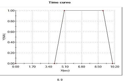
The CAD model seen in Fig. 1 is a mild steel plate developed using SOLIDWORKS Dassault 2021 for the investigation, with dimensions of 60 mm in length, 40 mm in breadth, and 10 mm in thickness. The simulation was conducted using the Thermal Simulation Program (TSP) within SOLIDWORKS Premium. The welding current (Amps), welding voltage (V), gas flow rate (liters/min), welding speed (mm/min), and welding temperature (°C) utilized in the analysis were derived from the research conducted by Bassey et al. [10], which focused on finite element simulation for the thermo-mechanical transient behaviour of mild steel plates joined by the GTAW technique. This study examined AISI 1018 mild steel plate, characterized by the mechanical properties and chemical contents detailed in Table 1. Table 2 delineates the specifics of the thermal loads employed in the investigation. Table 3 enumerates the specifics of the contacts utilized in the analysis. Table 4 presents details of the sensors used in the analysis. Table 5 presents details of the mesh used in the study.
Table 1. Properties and composition of AISI 1018 mild steel plate.
This table is shown in the PDF version of the article.
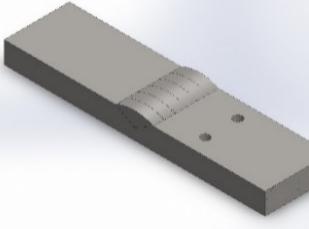
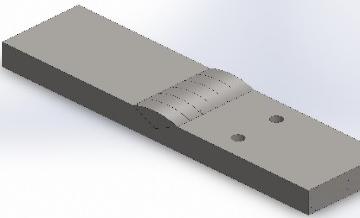
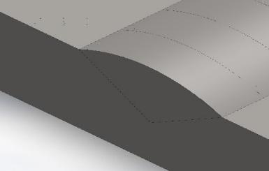
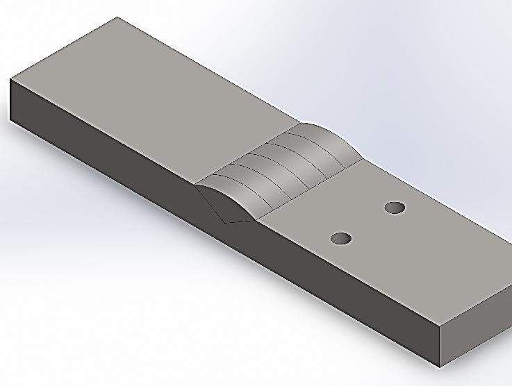
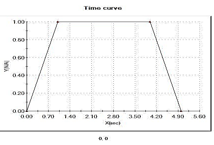
Table 2. Details of thermal loads employed in the analysis.
This table is shown in the PDF version of the article.
Table 3. Details of contact information employed in the analysis.
This table is shown in the PDF version of the article.
Table 4. Sensor details employed in the analysis.
This table is shown in the PDF version of the article.
Table 5. Mesh information employed in the analysis
This table is shown in the PDF version of the article.
% of elements with an aspect ratio < 3 99.7 % of elements with aspect ratio > 10 0 % of distorted elements (Jacobian) 0 Time to complete mesh (hh:mm: ss) 00:00:27
Mesh Control Name Mesh Control Image Mesh Control Details Control-1 Entities: 7 edge(s), 2 face(s) Units: mm Size: 0.332403 Ratio: 1.5
Control-2 Entities: 6 component(s) Units: mm Size: 0.664806 Ratio: 1.5
3. Thermal Equations
The gross energy input can be measured in two ways:
For a direct current, heat input (Qn) is calculated as the product of current and voltage at the arc, multiplied by the welding duration (t). In the instance of a sinusoidal alternating current, root mean square values of voltage and current and the power factor are employed for assessing the arc power. Three input parameters constituted the mathematical model for the heat source. The heat produced is described by Eq. (1).
60 × Amps × Volts
Heat Input = . (1)
in 1000 × Travel speed ( ) min To ensure simplicity, it was presumed that all experiments were conducted at an average welding velocity of 15 inches per minute (0.375 meters per minute). The gas served as a shielding mechanism against contaminants and mitigated heat loss; hence, the effectiveness of the process is contingent upon the gas flow rate. The gas flow rates were so changed to reflect the efficiency of the operation. Schnick et al. [14] asserted that the characteristics and flow rate of the shielding gas can enhance arc efficiency by 5-10%. Throughout the experiments, the arc length was preserved; hence, the gas flow rate served as a metric for assessing efficiency. The efficiency in question is immediate efficiency. The arc efficiencies were evaluated based on the gas flow rate. Standard gas flow rates ranged from 10 to 35 CFH (5 to 17 L/min), with associated arc efficiencies detailed in Table 6.
Table 6. Gas flow rate corresponding to arc efficiencies.
This table is shown in the PDF version of the article.
In structural mechanics, boundary conditions may be kinematic, with displacements specified at the conclusion of the simulation, or static, where response and consequent forces are observable throughout the simulation's progression. The designated temperature, heat flow, heat flux, or convection can be established by entering an initial set of values or process parameters into the computer-aided design program utilized for thermal analysis. Initial values may be provided in situations involving time. This study focused on transient thermal analysis to ascertain temperature variations and Coefficient of Thermal Expansion (CTE) under time-varying thermal loads. The welding process is deemed non-linear because of the temperature distribution on the material surface. Considering a function U(x, y, z, t) of three spatial variables (x, y, z) and the time variable t, the mathematical formulation of the heat equation for the welding condition is given by Eq. (2).
2 2 2
∂u ∂ u ∂ u ∂ u
− α ( + + ) = 0. (2)
2 2 2
∂t ∂x ∂y ∂z
In the physical condition of temperature variation, U(x, y, z, t) denotes the temperature while α denotes the thermal diffusivity. From Fourier’s law, the rate of flow of heat energy per unit area through the surface of the workpiece during welding operation is proportional to the negative temperature gradient across its surface, given by Eq. (3).
q = −k∇u. (3)
Where k is the thermal conductivity, and u is the temperature. In the absence of work done, the change in the internal energy per unit volume of the material (ΔQ) is proportional to the change in temperature (Δu) given by Eq. (4).
∆Q = cpρ∆u. (4)
Where cp is the specific heat capacity, and ρ is the mass density of the material. Selecting zero energy at absolute zero temperature can be expressed by Eq. (5).
Q = cpρu. (5)
When work is done in terms of welding operation and heat sources are present, the expression is given by Eq. (6).
x+∆x t+∆t x+∆x
c ρ ∫ [u(ξ, t + ∆t) − u(ξ, t − ∆t)] dξ = c ρ ∫ ∫ dξdτ. (6)
x−∆x t−∆t x−∆x ∂τ When no work is done, and there are no heat sources present, the change in internal energy in the interval (x−Δx, x+Δx) is accounted for by the flux of heat across the boundaries. Considering Fourier's law, this is given by Eq. (7).
t+∆t t+∆t x+∆x 2
∂u ∂u ∂ u
k ∫ [ (x + ∆x, τ) − (x − ∆x, τ)] dτ = k ∫ ∫ dξdr. (7)
t−∆t ∂x ∂x t−∆t x−∆x ∂ξ During the welding operation, temperature variation across the workpiece may result in expansion or contraction. Therefore, the thermal strain is given by Eq. (8).
εth = α∆T. (8)
Where, εth signifies the thermal strain, α signifies the CTE, and ∆T is the temperature variation. The thermal effects, as proposed by Hooks law, are given by the relationship in Eq. (9).
εxx −v −v σ 1 0 0 0 xx 1 εyy σ −v 1 −v 0 0 0 yy 1 εzz 1 −v 1 σ −v 0 0 0 zz 1
ϓ = + α∆T . (9)
xy 0 0 0 (1 + v) 0 0 σxy 0 ϓ 0 0 0 0 (1 + v) 0 σxz 0
xz
[ϓ ] [ 0 0 0 0 0 (1 + v)] [σyz] [0]
yz
The governing partial differential equation for the transient heat conduction is given by Eq. (10).
2 2 2 2 2 2
K(T) (∂ T/ ∂x ) + (∂ T/ ∂y ) + (∂ T/ ∂z ) + Q = ρ(T) CP(T) ) ∂T/ ∂t. (10)
Where x, y, and z represent the Cartesian coordinates, Q is the internal heat generated, ρ is the density, k is the thermal conductivity, and CP is the specific heat, are functions of the welding temperature (T). Given by Eq. (11), the heat loss by free convection is based on Newton’s law, where the coefficient of convective heat transfer is assumed to vary with both temperature and orientation of the boundary.
qc = (K Nu/L)(T − Ta). (11)
Where K represents the thermal conductivity of the material, L is the characteristic length of the mild steel plate, Ta is the ambient temperature, and Nu is the Nusselt number given by Eq. (12).
1/3 1/3 (12)
Nu = 5.67 Pr Gr .
Where Pr represents the Prandtl number and Gr is the Grashof number, both being functions of ambient air properties and temperature differences between the weldment and the environment. Heat loss as a result of radiation may be significant when the temperature difference between the weldments and the environment is high. This is given by the relation proposed by standard Stefan-Boltzman in Eq. (13).
qr = ε σ (T − Tα ). (13)
Where ε represents the heat emissivity, and σ is the Stephan-Boltzman constant. The total strain within the material after the TIG welding operation must satisfy the following compatibility conditions given by Eq. (14).
2 ′ 2 ′ 2 ′ 2 " 2 " 2 "
∂ εx ∂ εy ∂ γxy ∂ εx ∂ εy ∂ γxy
[ + − ] + [ + − ] = 0. (14)
2 2 2 2
∂y ∂x ∂x ∂y ∂y ∂x ∂x ∂y In the molten pool region of arc welding, the continuity equation for the incompressible fluid is given by Eq. (15).
1 ∂(xρv) ∂(ρu)
+ = 0. (15)
x ∂x ∂z Where ρ is the density of the fluid, v and u are the axial and radial velocity. Considering the axial momentum conservation equation, the molten metal in the weld pool and movement of argon shielding gas agrees with Eq. (16) and Eq. (17).
∂u ∂u ∂P ∂ ∂u 1 ∂ ∂u 1 ∂ ∂v
ρv + ρu = − + 2 (μ ) + (xμ ) + (xμ ) + j B + ρg. (16)
∂x ∂z ∂z ∂z ∂z x ∂r ∂x x ∂r ∂z From Eq. (16), the radial momentum conservation equation is given by the mathematical relationships in Eq. (17).
∂v ∂u ∂P 1 ∂ ∂v ∂ ∂v ∂u v
ρv + ρu = − + μ (2 (x ) + ( + ) − 2 − j B . (17)
2 z θ
∂x ∂z ∂x x ∂x ∂x ∂z ∂z ∂z x Where P is the pressure and μ the velocity flow of argon shielding gas used for the welding operation, Goldak et al. [15] developed a model to characterize the volumetric heat flux exerted on a plate by the welding arc heat in operations where the arc's momentum transfer impact on the weld pool is significant. In arc welding, precise outcomes are achieved via a power density distribution characterized by ellipsoidal surfaces with constant power density, where the power density along radial lines follows a Gaussian distribution. To address the disparity between the experimentally measured and predicted temperature gradients in front of and behind the arc, two ellipsoidal heat sources were agglutinated, as illustrated in Fig. 2; the anterior portion of the source comprises one quadrant of an ellipsoidal source, while the posterior portion consists of a quadrant from another ellipsoidal heat source.
The moving heat source was modeled according to the Goldak model. From the Goldak heat source model, the volumetric heat flux for a point in the domain Ω is given by Eq. (18) [16].
6 3Qr 2 2 2 √ f x y ξ exp [−3 ( + + )] for all (x, y, ξ ≥ 0) ∈ Ω
2 2 2
abc π√π a b c
qG(x, y, ξ) = . (18)
6√3Qr 2 2 2 r x y ξ exp [−3 ( + + )] for all (x, y, ξ < 0) ∈ Ω
2 2 2
{abc π√π a b c } Where rf and rr are the heat input proportions in the front and rear ellipsoid quadrants, is the energy input rate from the arc, abcr and cr represent the redii of the flux distribution. Transient heat conduction by the flat plate during the welding sequence is expressed by the linear partial differential equation given by Eq. (19):
2 (19)
ρc − k∇ T = q.
Where ρ, k and c denote the mass density, thermal conductivity, and specific heat capacity, and q is the rate of internal heat generation, which is considered an applied heat source. However, the natural boundary condition for conduction and radiation heat taking place in the welded material during the welding cycle is by Eq. (20).
k − q + h(T − To) + σε(T − To ) = 0. (20)
Where T denotes the temperature variable, q is the heat flux, h is the coefficient of heat conduction, σ is the melt pool emissivity, and ε is the Stephan-Boltzmann constant. The basic solution of the heat equation in one dimension is given by Green’s function in Eq. (21).
′ ′ 1 (x−x ) ′ ′
K(x − x , t − t ) = exp [− ] for all(x − x , t − t ≥ 0) ∈ Ω. (21)
′ 4α (t−t′) √4πα (t−t )
Where α is the thermal diffusivity given by Eq. (22):
α = . (22)
ρcp However, two and three-dimensional Green’s functions are obtained by multiplying one-dimensional Green’s functions by the Cartesian co-ordinates, of which the three-dimensional basic solution K(x-x’, y-y’, z-z’, t-t’) for the heat equation is given by Green’s function in Eq. (23).
′ 2 ′ 2 ′ 2
1 (x − x ) + (y − y ) + (z − z ) K = exp [− ] for all(x − x , y − y , z 3/2 ( ′)
′ 4α t − t (23)
(4πα(t − t )) − z , t − t ≥ 0 ∈ Ω).
If only conduction is being considered, the weldment can be modelled by considering insulating boundary conditions at every face. In three dimensions, it can be shown, via the Laplace transform method, that the Green’s function that describes this, G(x-x’, y-y’, z-z’, t-t’), is given by Eq. (24).
n =∞ ′ 2 ′ 2
1 (2n B + x − x ) (2n B + x + x ) ∑ [exp[− ] + exp[− ]] ( ′) ( ′) n =−∞ 4α t − t 4α t − t
n =∞ ′ 2 ′ 2
1 2 (2n D + y − y ) (2n D + y + y )
G = x ∑ [exp[− ] + exp[− ]] . (24)
3/2 ( ′) ( ′) ′ n =−∞ 4α t − t 4α t − t (4πα(t − t )) 2
n =∞ ′ 2 ′ 2
3 (2n L + z − z ) (2n L + z + z ) x ∑ [exp[− ] + exp[− ]] ( ′) ( ′) n =−∞ 4α t − t 4α t − t { 3 } During welding operation, temperature variation across the workpiece may result in expansion or retraction. B, D and L are the spatial extent of the plate in the x, y and z directions, respectively. The thermal reaction resulting from solid-to-liquid phase transformation can be due to an increase in specific heat (Cp) input in the temperature between solidus and liquidus temperature range. In the welding process, latent heat of fusion is released in the phase transformation, thus causing the increase in the enthalpy (h) [17] given by Eq. (25).
h = ρCpT + ρLff ρCpT. (25)
Where the latent heat of fusion is denoted by Lf, ρ is the density, f is the mass proportion of molten metal in the weldment, and Cp′ is the increased specific heat. In the welding process, ρ is assumed as constant, and f is given by Eq. (26), [18].
(26)
When the temperature ranges from solidus to liquidus temperature, the equivalent specific heat Cp is deduced from Eq. (27).
L T − Ts
Cp = Cp + . (27)
T TL − Ts Also, if the temperature of the weld pool is above the melting point, the latent heat of evaporation (Le) can be considered in the FE model by using the equivalent specific heat Cp given by Eq. (28).
Le T − Tb
Cp = Cp + . (28)
T Tmax − Tb The distribution of heat across the weld region is characterised by a non-linear flow pattern due to the dependence of material thermo-physical properties on the welding temperature. Consequently, the heat diffusion equation is given by Eq. (29).
∂T ∂ ∂T ∂ ∂T ∂ ∂T
ρ(T) c(T) = q + (Kx(T) ) + (Ky(T) ) + (Kz(T) ). (29)
∂t ∂x ∂x ∂y ∂y ∂z ∂z where ρ(T) is the mass density, c(T) is the specific heat, q is the heat generated per unit volume, Kx(T), Ky(T), and Kz(T) are the thermal conductivity coefficients in each direction, T is temperature and t is time. Considering that enthalpy is given by Eq. (30), the formulation of enthalpy for heat diffusion is expressed in Eq. (31).
H = ∫ ρ(T) c(T)dT. (30)
∂H ∂ ∂T ∂ ∂T ∂ ∂T
= q + (Kx(T) ) + (Ky(T) ) + (Kz(T) ). (31)
∂t ∂x ∂x ∂y ∂y ∂z ∂z
4. Discussion
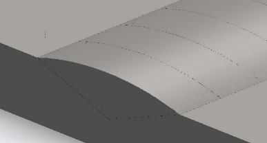
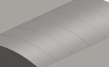
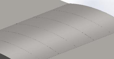
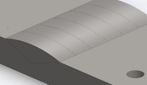
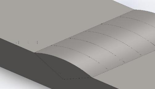
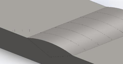
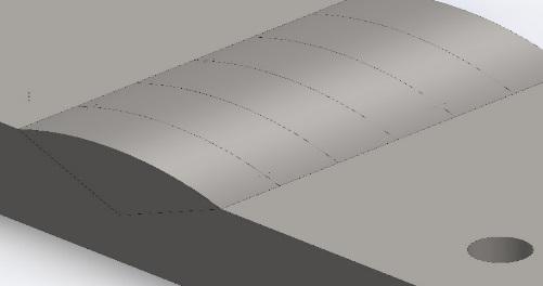
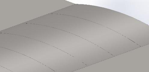
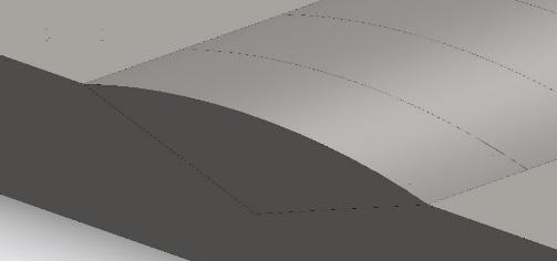
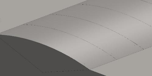
The distribution of heat input across the weld zone plays a crucial role in determining the mechanical properties and integrity of the weld. The parameters of the heat distribution, including the depth and size of the heat application region, as well as its intensity, were modified to achieve an adequate correlation with the thermal information reported by Depradeux [19]. According to this information, the heat that was applied was distributed evenly across two planes of the plate: the upper face and the other plane that is parallel to it. This study focused on the heat input distribution profile on the upper face of the weld and a parallel plane positioned 1.5 mm below the upper face (see Fig. 3 and Fig. 4).
The upper face of a weld refers to the surface of the weld that is exposed to the heat source during the welding process, while the parallel plane located 1.5 mm below the upper face represents a critical region in the weld zone where the heat input can have a significant impact on the mechanical properties of the weld. The heat input distribution profile on the upper face of a weld is typically characterized by a peak in heat input at the centre of the weld, which gradually decreases towards the edges of the weld. This distribution profile is influenced by various factors, including the welding parameters (such as welding current, voltage, and travel speed), the geometry of the weld joint, and the properties of the base metal. On the other hand, the heat input distribution profile on the parallel plane located 1.5 mm underneath the upper face may exhibit a different profile pattern compared to the upper face, as clearly seen in Fig. 3 and Fig. 4. This is because the heat input at this depth is influenced by factors such as heat conduction through the base metal, the presence of any heat sinks or thermal barriers, and the thermal conductivity of the base metal. It can be observed that the distribution of the heat input looks like a Gaussian distribution, as shown in Fig. 3 and Fig. 4.
Since the welded metal plate had finite dimensions around the edge regions, there was an occurrence of intense heat concentration as a result of heat transfer by convection on the edges, which was compared to the transfer by conduction in the bulk of the plate [20]. Understanding the heat input distribution profile on both the upper face and the parallel plane located 1.5 mm below the upper face is essential for ensuring the quality and integrity of a weld. A uniform distribution of heat input across the weld zone can help prevent defects such as weld cracking, distortion, and poor mechanical properties. Therefore, it is important for welders to carefully control the welding parameters and techniques to achieve a desirable heat input distribution profile.
Weld profile simulation is a crucial aspect of welding processes, as it allows for the prediction and analysis of various parameters, such as CTE and TTV in mild steel plates. This plays a vital role in addressing weld defects as well as factors that hamper the quality and performance of a welded joint. The CTE of mild steel plates can vary depending on the specific composition of the material. This variation in CTE can bring about challenges such as residual stresses, distortion, and cracking in the welded joint. To address the aforementioned challenges, the weld profile must be simulated in order to predict the variations in transient temperature during the welding sequence. Simulation of weld profiles enables welding practitioners to control and optimize the welding parameters in order to minimize the effects of CTE around the weld region and obtain the required mechanical properties.
The FEM approach was employed in this simulation due to its capacity to model complex physical phenomena accurately. The principles behind the computational modelling of weld profiles involve the application of mathematical models in representing the thermal variations and material response during the welding sequence [21].
By inputting parameters such as welding voltage, welding current, gas flow rate and material properties, the simulation can predict the temperature distribution and resulting weld profile. Heat conduction theory is employed in computing the temperature variations within the weld profile model, while thermal expansion theory is used for predicting the CTE in relation to the welding temperature across the weld profile model. Figs. 5, 7, 9, 11, 13 and 15 represent weld profiles at maximum temperatures of 1391, 1516, 1667, 2200, 2596 and 2834 oC. However, Fig. 6, 8, 10, 12, 14 and 16 represent weld profiles for CTE at the same maximum temperature regeems. It is clearly observed from these profiles that maximum weld temperatures in Figs. 5-15 yieded corresponding maximum CTE of 1.1e-014, 1.1e-012, 1.1e-011, 1.1e-009, 1.1e-007 and 1.1e-005 oC-1 as shown in Figs. 6-16. Critically observing the trend of these values, it was deduced that increasing weld temperatures can obviously result in increasing CTE. Therefore, the higher the weld temperature, the higher the CTE. These agree with the findings of Depradeux [19] and Bezerra et al. [22].
It should be noted that extremely high welding temperatures can lead to grain growth, phase transformations, and the formation of undesirable phases, particularly when the CTE of the welded metal is exceeded, all of which can affect the strength and toughness of the weld. By simulating the temperature variations in the weld zone using FEM, adequate predictions can be made on the evolution of the microstructure and the welding parameters tailored to achieve the desired mechanical properties in the output weld.
Dynamic viscosity is an important parameter in the welding field, which directly influences the flow behaviour of molten metal during the welding process. When considered in the context of welding, dynamic viscosity is the resistance of molten metal to flow during the welding application and is widely influenced by factors such as temperature, pressure, and composition [23]. During the welding procedure of a mild steel plate, the dynamic viscosity of the molten metal plays a vital role in terms of the weld quality.
Fig. 17 illustrates the relationship between dynamic viscosity and welding temperature of mild steel plate. From the graphical illustration, the dynamic viscosity of the molten metal gradually decreases as the welding temperature increases. This is a result of the decrease experienced by the viscosity of the molten metal due to a higher temperature gradient, accelerating the melting process and enabling the molten metal to overcome the flow resistance to occupy the weld joint. The plot obviously indicates an inverse relationship between the two parameters, implying a decrease in the dynamic viscosity of the molten metal when the welding temperature increases. This has a significant effect on the welding sequence as it suggests that higher welding temperatures can result in improved flow characteristics of the molten metal and possibly standard weld quality.
Therefore, increasing the welding temperature within a specific range can enable welding practitioners to improve the flow condition of the molten metal, thereby minimizing the likelihood of welding defects around the fusion zones. Understanding the relationship between these two parameters is crucial for achieving the desired weld quality.
0/008 1391 ؛0/0074 0/007 1516 ؛0/0062 0/006 1667 ؛0/0052 0/005
0/004 2200 ؛0/0035
Dynamic Viscosity (Pa*s) 0/003 2834 ؛0/0024
2596 ؛0/0027 0/002 1000 1500 2000 2500 3000
Welding Tempeature (oC)
In the welding context, specific heat relates to the extent of heat input needed to increase the temperature of a unit mass of the welded metal by one degree Celsius. Therefore, it plays a vital role in the determination of temperature distribution across the weld fusion zones. This is crucial when welding mild steel plates, as plotting specific against welding temperature indicates thermal response and variations of the metal during the welding sequence. For example, a steep increase in specific heat at higher temperatures may signify the beginning of phase transformations or other metallurgical variations that could directly or indirectly influence the grain size, phase transformation, microstructure, mechanical properties and compositions of the weld [24], [25]. The relationship between these parameters provides valuable insights into the thermal characteristics (heat input and energy transfer) of the welded metal during the welding sequence.
Fig. 18 illustrates the relationship between specific heat and welding temperature of mild steel plates. From the plot, a higher specific heat value is an indication that more heat input has been introduced to increase the temperature of the welded metal due to higher welding temperature, which improves the thermal behaviour of the welded material. On the other hand, a lower specific heat value signifies that less amount of heat has been introduced to the welding sequence, resulting in a lower welding temperature. In other words, the relationship between these parameters illustrates how rapidly the temperature accelerates and how efficiently heat is transferred across the welded metal as a result of increasing welding temperature. This, in turn, influences the geometry of the HAZ in terms of size and shape, as well as the strength and integrity of the weld. Understanding the relationship between these parameters can enable welding practitioners to optimize the welding conditions to achieve optimum microstructural changes and better weld quality while minimizing the risk of defects such as cracking and distortion.
2834 ؛1862
1600 2596 ؛1593
2200 ؛1349
Specific Heat (J/kg*oC) 1667 ؛1180
1516 ؛1140 1100 1391 ؛1123
1200 1400 1600 1800 2000 2200 2400 2600 2800 3000
Welding Temperature (oC)
Energy consumption is a crucial parameter in welding operations due to its impact on the efficiency and cost-effectiveness of the welding sequence. During the welding sequence, the temperature plays a major role in the determination of the energy consumption. In other words, energy consumption in TIG welding is mainly determined by the heat input required to melt the base metal and filler material. The temperature of the welding process directly influences the heat input, as higher temperatures require more energy to melt the materials [26], [27]. As a result, there is a direct correlation between the welding temperature and the energy consumption.
Fig. 19 shows the relationship between energy consumption and welding temperature of mild steel plates. The plot illustrates an increasing trend, as increasing welding temperatures result in increasing energy consumption, indicating that higher temperatures require more energy to melt the metal, which ultimately results in increased energy consumption. Moreover, the efficiency of the welding process may decrease at peak temperatures, further contributing to the increase in energy consumption.
High energy consumption during TIG welding can result in extreme heat input, which may cause undesirable microstructural variations on the fusion and HAZs. This can further cause a reduction of tensile strength and ductility of the weld. On the other hand, low energy consumption can lead to insufficient heat input, causing incomplete fusion as well as improper weld penetration. This can cause improper bonding between the base metal and the filler material, resulting in weak weld joints. It is crucial to achieve a balance between high and low energy input during TIG welding of mild steel plates. Therefore, the energy input should be enough to obtain optimum temperature for adequate weld bead penetration while avoiding intensive heat input that can result in the formation of undesirable microstructures. Optimum energy consumption can be achieved by controlling the welding parameters, such as welding current, welding speed, and shielding gas flow rate. 900 2834 ؛903 2596 ؛874
2200 ؛820
750 1667 ؛749 1516 ؛724 700 1391 ؛702
Energy Consumption (kW/h)
1200 1400 1600 1800 2000 2200 2400 2600 2800 3000
Welding Temperature (oC)
Mild steel is a commonly used material in welding applications due to its excellent weldability and mechanical properties. The thermal conductivity of mild steel is relatively high compared to other materials, which means that it can conduct heat efficiently [28]. As the welding temperature increases, the thermal conductivity of the material also increases, leading to a more uniform distribution of heat within the material [29]. This can be clearly observed in Fig. 20, as it clearly illustrates the relationship between thermal conductivity and welding temperature, which the physical mechanisms of heat transfer in the material can describe. At low temperatures, heat is primarily transferred through conduction, where the temperature gradient within the material drives the movement of heat. As the temperature increases, other modes of heat transfer, such as convection and radiation, become more effective, causing thermal variations around the fusion zone and HAZ of the weld. During welding sequence, the HAZ of the weld undergoes intense variations in microstructure and mechanical properties due to the heat input during welding [30]. A critical assessment of the thermal welding parameters such as heat input, welding speed, and preheating temperature can identify the temperature range at which the HAZ is formed and as well as its overall impact on the weld quality. Thereafter, the welding materials can be adjusted to suit the material’s requirement in order to minimize the formation of welding defects such as cracks, porosity, and distortion in the welded joint.
0/21 1391 ؛0/2 0/19 1516 ؛0/185 0/17 1667 ؛0/17 0/15 0/13 2200 ؛0/12 0/11 0/09 2596 ؛0/09 0/07 2834 ؛0/07
Thermal Conductivity (W/m*oC)
0/05 1200 1400 1600 1800 2000 2200 2400 2600 2800 3000
Welding Temperature (oC)
5. Conclusion
The findings from this study provided valuable insights into the relationship between the CTE and TTVs in mild steel plates. Through the use of advanced computational tools, this study simulated and analyzed the complex interactions that occur during the welding sequence, leading to a better comprehension of the factors that influence weld quality and performance. One of the key findings from this study included the impact of CTE on TTVs in the weld profile. It was observed that variations in the CTE can cause non-uniform heating and cooling patterns in the weld zone, resulting in the formation of undesirable defects such as porosity and cracking. By accurately modelling these thermal effects, this study, through computational modelling simulated the weld profiles at different temperature conditions, and the outcomes were reported adequately. Furthermore, the findings from these studies have also highlighted the importance of considering the material properties of the base metal when preparing the welding sequence. Mild steel, for example, exhibits a specific CTE that must be taken into account when predicting temperature variations in the weld zone. By incorporating this information into computational models, the weld profile behavior can be predicted accurately and informed decisions can be made on the process parameters. Furthermore, this study also demonstrated the importance of accurately modelling the heat transfer mechanisms in TIG welding, as small variations in temperature can have a significant impact on the final weld quality. By integrating the welding parameters (welding current (Amps), welding voltage (V), gas flow rate (litters/min), welding speed (mm/min) and welding temperature (oC) and essential boundary conditions into the computational simulations, the analysis predicted the formation of key features in the weld profile, such as the heat input distribution profile on the upper face and parallel plane located 1.5 mm underneath the upper face, CTE, TTVs, heat-affected zone and fusion zone, with a high degree of accuracy. By leveraging the knowledge presented in this study, welding practitioners can continue to improve welding sequence and enhance the quality and reliability of welded structures.
Authors Contributions
Aniekan Ikpe: Conceptualization, modeling and simulation; Imoh Ekanem: Writing, review and editing; Jephtar Ohwoekevwo: Analysis of results. All authors have read and approved the manuscript.
Funding
The authors received no funding for the research study. All data supporting the reported findings in this research paper are provided in the paper. All authors have read and agreed to the publication of this research work.
Conflicts of Interest
The authors declare that there is no conflict of interest in this research paper. There was no second or third party involved in any part of this work or decision-making of the publication.
Figures

The PDF also contains 27 images in a format that could not be extracted automatically.
References
- [1] Arora, H., Singh, R., & Brar, G. S. (2019). Thermal and structural modelling of arc welding processes: A literature review. Measurement and control, 52(7–8), 955–969. https://doi.org/10.1177/0020294019857747
- [2] Zhang, Y. M., Yang, Y. P., Zhang, W., & Na, S. J. (2020). Advanced welding manufacturing: A brief analysis and review of challenges and solutions. Journal of manufacturing science and engineering, 142(11). https://doi.org/10.1115/1.4047947
- [3] Hanninen, H., Aaltonen, P., Brederholm, A., Ehrnstén, U., Gripenberg, H., Toivonen, A., ... & Virkkunen, I. (2006). Dissimilar metal weld joints and their performance in nuclear power plant and oil refinery conditions. VTT tiedotteita, 2347(208). https://b2n.ir/q81932
- [4] Mohajernia, B., & Urbanic, J. (2023). Exploring computational techniques for simulating residual stresses for thin wall multi-joint hexagon configurations for a laser directed energy deposition process. The international journal of advanced manufacturing technology, 126(5), 2745–2763. https://doi.org/10.1007/s00170-023-11145-2
- [5] Verma, J., & Taiwade, R. V. (2017). Effect of welding processes and conditions on the microstructure, mechanical properties and corrosion resistance of duplex stainless steel weldments-A review. Journal of manufacturing processes, 25, 134–152. https://doi.org/10.1016/j.jmapro.2016.11.003
- [6] Singh, D. K., Sharma, V., Basu, R., & Eskandari, M. (2019). Understanding the effect of weld parameters on the microstructures and mechanical properties in dissimilar steel welds. Procedia manufacturing, 35, 986–991. https://doi.org/10.1016/j.promfg.2019.06.046
- [7] Ikpe, A. E., & Bassey, M. O. (2023). Modelling and simulation of transient thermal stress distribution across AISI 1018 flat plates at variable welding temperature regime. Journal of materials engineering, structures and computation, 2(3). https://doi.org/10.5281/zenodo.8297860
- [8] Huang, H., Yin, X., Feng, Z., & Ma, N. (2019). Finite element analysis and in-situ measurement of out-of-plane distortion in thin plate TIG welding. Materials, 12(1). https://doi.org/10.3390/ma12010141
- [9] Aissani, M., Guessasma, S., Zitouni, A., Hamzaoui, R., Bassir, D., & Benkedda, Y. (2015). Three-dimensional simulation of 304L steel TIG welding process: contribution of the thermal flux. Applied thermal engineering, 89, 822–832. https://doi.org/10.1016/j.applthermaleng.2015.06.035
- [10] BASSEY, M., Offiong, U., & Ikpe, A. (2023). Finite element simulation for thermo-mechanical transient behavior of mild steel plate agglutinated by gas tungsten arc welding (GTAW) technique. Journal of materials engineering, structures and computation, 2(3), 549–559. https://doi.org/10.5281/zenodo.8306756
- [11] Nezamdost, M. R., Esfahani, M. R. N., Hashemi, S. H., & Mirbozorgi, S. A. (2016). Investigation of temperature and residual stresses field of submerged arc welding by finite element method and experiments. The international journal of advanced manufacturing technology, 87(1), 615–624. https://doi.org/10.1007/s00170-016-8509-4
- [12] Beygi, R., Marques, E., & da Silva, L. F. (2022). Computational concepts in simulation of welding processes. Springer international publishing. http://dx.doi.org/10.1007/978-3-030-97910-2
- [13] Bassey, M. O., Ohwoekevwo, J. U., & Ikpe, A. E. (2024). Thermal analysis of AISI 1020 low carbon steel plate agglutinated by gas tungsten arc welding technique: a computational study of weld dilution using finite element method. Journal of engineering and applied science, 71(1), 33. https://doi.org/10.1186/s44147-024-00375-0
- [14] Schnick, M., Dreher, M., Zschetzsche, J., Füssel, U., & Spille-Kohoff, A. (2012). Visualization and optimization of shielding gas flows in arc welding. Welding in the world, 56(1), 54–61. https://doi.org/10.1007/BF03321146
- [15] Goldak, J., Chakravarti, A., & Bibby, M. (1984). A new finite element model for welding heat sources. Metallurgical transactions b, 15(2), 299–305. https://doi.org/10.1007/BF02667333
- [16] Anie, C. O. (2018). Evaluation of biofilm and enterotoxin producing capacity of methicillin-resistant Staphylococcus aureus isolated from healthy person. Journal of applied sciences and environmental management, 22(12), 1881–1884. https://doi.org/10.4314/jasem.v22i12.2
- [17] Cho, J., & Na, S. J. (2009). Three-dimensional analysis of molten pool in GMA-laser hybrid welding. Welding journal (Miami, Fla), 88, 35s-43s. https://B2n.ir/jn7551
- [18] Piekarska, W., & Kubiak, M. (2011). Three-dimensional model for numerical analysis of thermal phenomena in laser–arc hybrid welding process. International journal of heat and mass transfer, 54(23), 4966– 4974. https://doi.org/10.1016/j.ijheatmasstransfer.2011.07.010
- [19] Depradeux, L. (2004). Simulation numérique du soudage-acier 316l: validation sur cas tests de complexité croissante. [Thesis]. https://theses.fr/2004ISAL0014
- [20] Bezerra, A. C., Rade, D. A., & Scotti, A. (2005). Finite element simulation of tig welding: thermal analysis. In 18th international congress of mechanical engineering. https://www.academia.edu/download/81246307/COBEM2005-0866.pdf
- [21] Malik, V., Sanjeev, N. K., & Bajakke, P. (2020). Review on modelling of friction stir welding using finite element approach and significance of formulations in simulation. International journal of manufacturing research, 15(2), 107–135. https://doi.org/10.1504/IJMR.2020.106851
- [22] Bezerra, A. C., Rade, D. A., & Scotti, A. (2005). Finite element simulation of tig welding: structural analysis [presentation]. International congress of mechanical engineering, cobem, ouro preto. https://www.academia.edu/download/115650766/COBEM2005-0867.pdf
- [23] Fotovvati, B., Wayne, S. F., Lewis, G., & Asadi, E. (2018). A review on melt-pool characteristics in laser welding of metals. Advances in materials science and engineering, 2018(1), 4920718. https://doi.org/10.1155/2018/4920718
- [24] Raju, S., B, J., Tripathy, H., Murugesan, S., Saibaba, S., Albert, S. K., & Bhaduri, A. K. (2016). Thermal stability, phase transformation characteristics, and thermal properties of T91 steel and welding consumables. Welding in the world, 60(5), 963–977. https://doi.org/10.1007/s40194-016-0353-5
- [25] Singh, V. P., Patel, S. K., & Kuriachen, B. (2021). Mechanical and microstructural properties evolutions of various alloys welded through cooling assisted friction-stir welding: A review. Intermetallics, 133, 107122. https://doi.org/10.1016/j.intermet.2021.107122
- [26] Rosli, N. A., Alkahari, M. R., Abdollah, M. F. bin, Maidin, S., Ramli, F. R., & Herawan, S. G. (2021). Review on effect of heat input for wire arc additive manufacturing process. Journal of materials research and technology, 11, 2127–2145. https://doi.org/10.1016/j.jmrt.2021.02.002
- [27] Ikechukwu, O., & Aniekan E., İ. (2019). Finite element analysis of tungsten inert gas welding temperatures on the stress profiles of AIS1 1020 low carbon steel plate. International journal of engineering technologies IJET, 5(2), 50–58. https://dergipark.org.tr/en/pub/ijet/issue/45163/402386
- [28] Wu, S., Yan, T., Kuai, Z., & Pan, W. (2020). Thermal conductivity enhancement on phase change materials for thermal energy storage: A review. Energy storage materials, 25, 251–295. https://doi.org/10.1016/j.ensm.2019.10.010
- [29] Ekanem, I. I., Ohwoekevwo J. U, Achebo J. I, & Obahiagbon K. O. (2023). Back propagation neutral network based modelling and optimization of thermal conductivity of mild steel welds Agglutinated by Tungsten Inert Gas welding technique. Journal of materials engineering, structures and computation, 2(3 SE-Articles). https://doi.org/10.5281/zenodo.8310192
- [30] Ikechukwu, O., & Ikpe, A. (2019). Evaluation of induced residual stresses on AISI 1020 low carbon steel plate from experimental and FEM approach during TIG welding process. Journal of mechanical engineering and sciences, 13, 4415–4433. http://dx.doi.org/10.15282/jmes.13.1.2019.06.0376